Using birthweight data from the MASS library we will work through evaluating different modeling specifications:
library(MASS) # birthwt dataset
library(texreg) # for nice looking tables
library(tidyverse)
## Warning: package 'ggplot2' was built under R version 3.6.2## Warning: package 'tibble' was built under R version 3.6.2## Warning: package 'dplyr' was built under R version 3.6.2We will use the birthweight data to explore different model specifications. Here, bwt is the outcome variable of interest, birthweight.
head(birthwt)## low age lwt race smoke ptl ht ui ftv bwt
## 85 0 19 182 2 0 0 0 1 0 2523
## 86 0 33 155 3 0 0 0 0 3 2551
## 87 0 20 105 1 1 0 0 0 1 2557
## 88 0 21 108 1 1 0 0 1 2 2594
## 89 0 18 107 1 1 0 0 1 0 2600
## 91 0 21 124 3 0 0 0 0 0 2622The race variable is mother’s race and is coded:
- 1: White
- 2: Black
- 3: Other
Let’s make a new variable with more informative labels.
birthwt <- birthwt %>%
  mutate(race_fct = recode(race, `1` = 'White', `2` = 'Black', `3` = 'Other'))
# specify factor variable with White as reference category
birthwt$race_fct <- factor(birthwt$race_fct, levels = c('White', 'Black', 'Other'))
#check variable
table(birthwt$race, birthwt$race_fct)
##
## White Black Other
## 1 96 0 0
## 2 0 26 0
## 3 0 0 67Let’s explore what some of the predictor variables look like.
ggplot(data = birthwt, aes(x = age, y = bwt)) +
  geom_point() +
  geom_smooth(method=lm,se=F) +
  theme_bw()
## `geom_smooth()` using formula 'y ~ x'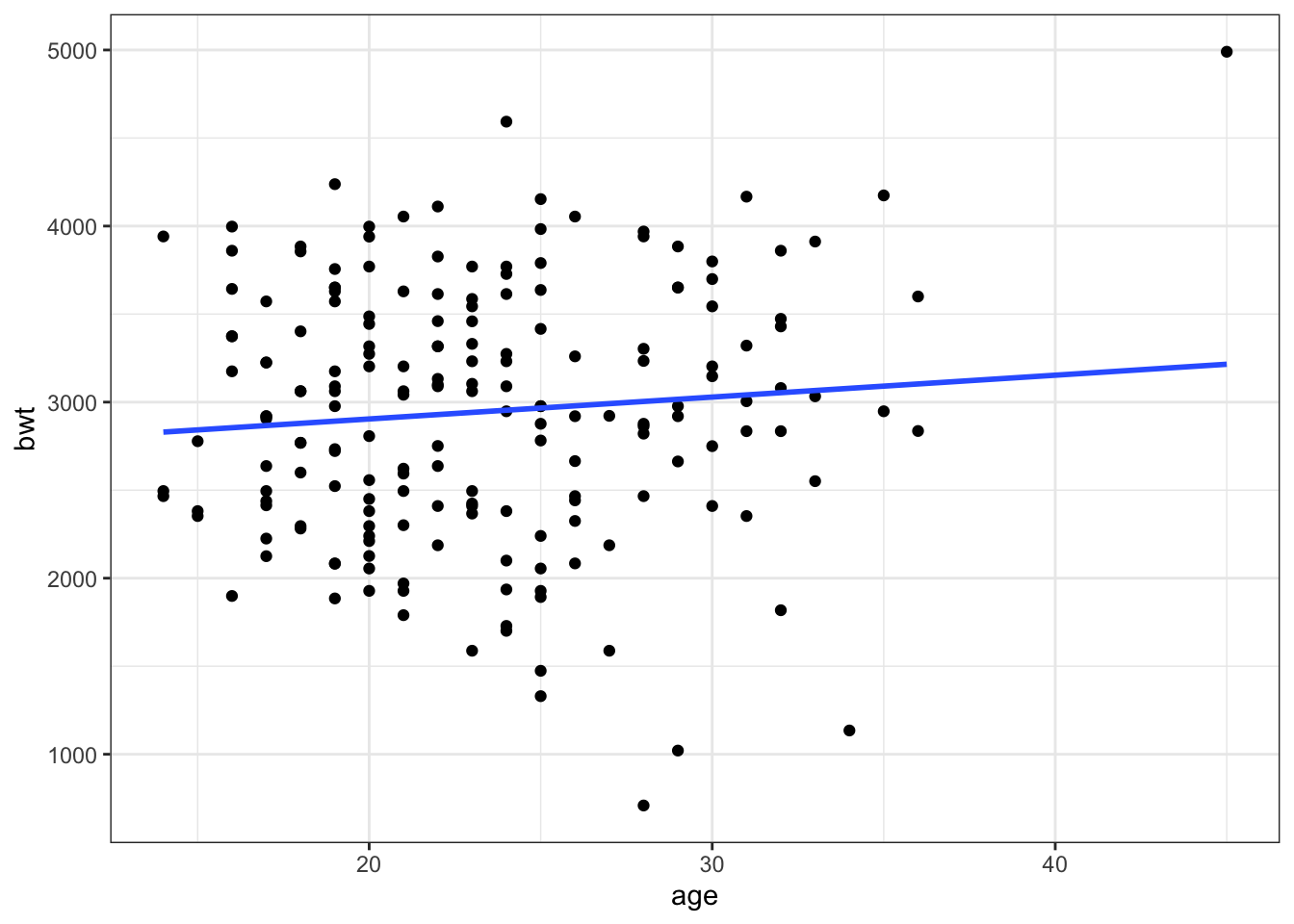
Figure 1: Age Plot
ggplot(data = birthwt, aes(x = age, y = bwt, color = race_fct)) +
  geom_point() +
  geom_smooth(method=lm,se=F) +
  theme_bw()
## `geom_smooth()` using formula 'y ~ x'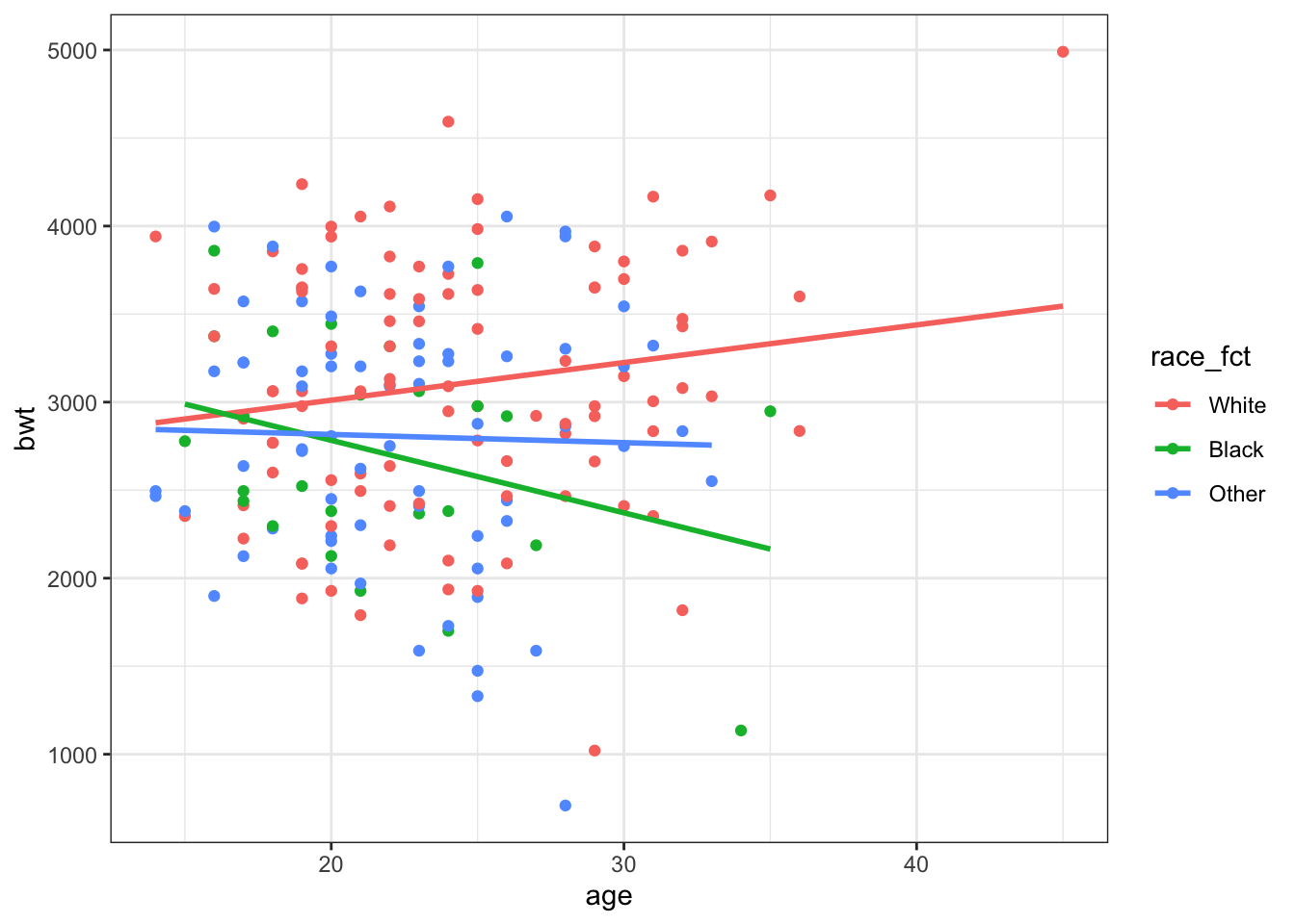
Figure 2: Age and Race Plot
The initial Figure 1 seems to suggest there is not much relationship (or maybe slightly positive) between age and birthweight. However, when we look at Figure 2, age by race, there seems to be different relationships across groups suggesting an interation between these predictors.
ggplot(data = birthwt, aes(x = smoke, y = bwt)) +
  geom_point() +
  geom_smooth(method=lm,se=F) +
  theme_bw()
## `geom_smooth()` using formula 'y ~ x'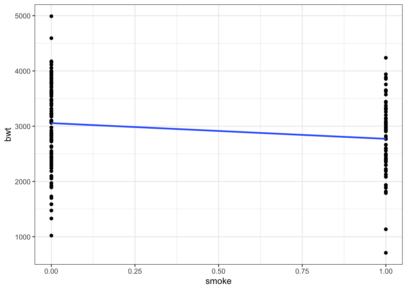
ggplot(data = birthwt, aes(x = smoke, y = bwt, color= race_fct)) +
  geom_point() +
  geom_smooth(method=lm,se=F) +
  theme_bw()
## `geom_smooth()` using formula 'y ~ x'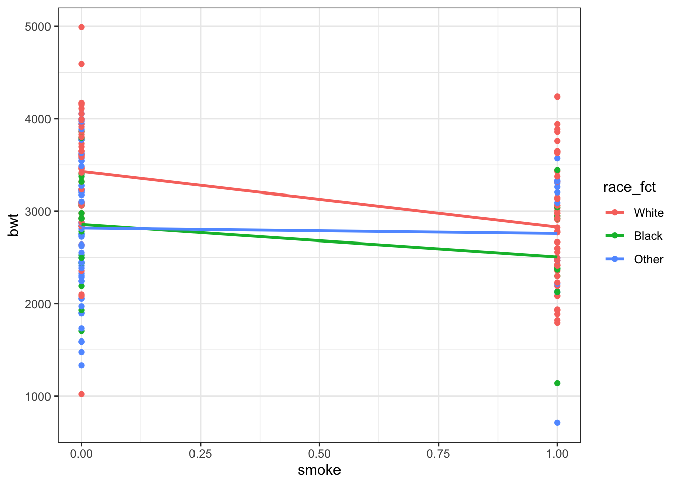
Looking at the relationship between smoking and birthweight in general there seems to be a negative relationship. But again, there might be an interactive effect with race.
Let’s compare different linear model specifications:
m1 <- lm(bwt ~ age + smoke, data = birthwt)
m2 <- lm(bwt ~ age + smoke + race_fct, data = birthwt)
htmlreg(list(m1,m2),doctype = F)| Model 1 | Model 2 | |
|---|---|---|
| (Intercept) | 2791.22*** | 3281.67*** |
| (240.95) | (260.66) | |
| age | 11.29 | 2.13 |
| (9.88) | (9.77) | |
| smoke | -278.36* | -426.09*** |
| (106.99) | (109.99) | |
| race_fctBlack | -444.07** | |
| (156.19) | ||
| race_fctOther | -447.86*** | |
| (119.02) | ||
| R2 | 0.04 | 0.12 |
| Adj. R2 | 0.03 | 0.10 |
| Num. obs. | 189 | 189 |
| ***p < 0.001; **p < 0.01; *p < 0.05 | ||
Including race of the mother, which we know from the health disparities literature in the United States is substantively important, is also statistically significant. In addition, we see that that the adjusted R squared has increased and the root mean squared error (RMSE) has decreased.
Adding in interactions:
m3 <- lm(bwt ~ age*race_fct + smoke, data = birthwt)
m4 <- lm(bwt ~ age*race_fct + smoke*race_fct, data = birthwt)
htmlreg(list(m1,m2,m3,m4),doctype = F)| Model 1 | Model 2 | Model 3 | Model 4 | |
|---|---|---|---|---|
| (Intercept) | 2791.22*** | 3281.67*** | 3032.07*** | 3251.05*** |
| (240.95) | (260.66) | (338.74) | (353.34) | |
| age | 11.29 | 2.13 | 11.60 | 6.83 |
| (9.88) | (9.77) | (12.85) | (12.98) | |
| smoke | -278.36* | -426.09*** | -389.78*** | -580.08*** |
| (106.99) | (109.99) | (113.67) | (146.58) | |
| race_fctBlack | -444.07** | 394.58 | 256.56 | |
| (156.19) | (699.09) | (705.20) | ||
| race_fctOther | -447.86*** | -61.30 | -332.36 | |
| (119.02) | (541.85) | (554.01) | ||
| age:race_fctBlack | -37.46 | -39.59 | ||
| (30.69) | (32.12) | |||
| age:race_fctOther | -15.87 | -11.43 | ||
| (22.74) | (22.70) | |||
| race_fctBlack:smoke | 365.94 | |||
| (336.12) | ||||
| race_fctOther:smoke | 522.09* | |||
| (263.26) | ||||
| R2 | 0.04 | 0.12 | 0.13 | 0.15 |
| Adj. R2 | 0.03 | 0.10 | 0.10 | 0.11 |
| Num. obs. | 189 | 189 | 189 | 189 |
| ***p < 0.001; **p < 0.01; *p < 0.05 | ||||
Based on the adjusted R squared and RMSE it looks like including age and smoke as interactions with race make for the best fitting model.
While, including additional predictors can improve model fit it can also lead to overfitting. One way to approach this is to separate your data into a training set and a test set. Use the training set to fit the model and then look at how well the model works on the out-of-sample (test) data. A model that is not overfit will continue to perform well.
Usually, we would want to randomly separate the data into a training and test set.
set.seed(12345)
# randomly draw row numbers 80% for training set, 20% for test set
train_obs <- sample(x=1:nrow(birthwt),size=.8*nrow(birthwt),replace = F)
train <- birthwt[train_obs,]
test <- birthwt[-train_obs,]
However, in order to demonstrate how overfitting can be a problem I’m going to separate into a very small training set.
train_obs <- c(1,2,3,29,42,57,140,152,138,165,167,184)
train <- birthwt[train_obs,]
test <- birthwt[-train_obs,]
Now, we fit our models on the training data and choose our preferred model.
m_train <- lm(bwt ~ age*race_fct + smoke*race_fct, data = train)
m_train1 <- lm(bwt ~ age + smoke, data = train)
m_train2 <- lm(bwt ~ age + smoke + race_fct, data = train)
htmlreg(list(m_train, m_train1, m_train2),doctype = F)| Model 1 | Model 2 | Model 3 | |
|---|---|---|---|
| (Intercept) | 17145.00 | 2156.67* | 2174.26* |
| (16560.35) | (772.11) | (842.86) | |
| age | -767.00 | 9.48 | 5.44 |
| (871.30) | (33.09) | (37.22) | |
| race_fctBlack | -15246.07 | -23.62 | |
| (16684.66) | (393.45) | ||
| race_fctOther | -15860.41 | 243.91 | |
| (16652.40) | (397.39) | ||
| smoke | 752.00 | 192.37 | 182.26 |
| (1444.88) | (301.00) | (328.89) | |
| age:race_fctBlack | 776.91 | ||
| (876.18) | |||
| age:race_fctOther | 809.27 | ||
| (873.55) | |||
| race_fctBlack:smoke | -260.96 | ||
| (1571.43) | |||
| race_fctOther:smoke | 58.11 | ||
| (1679.96) | |||
| R2 | 0.52 | 0.04 | 0.12 |
| Adj. R2 | -0.76 | -0.17 | -0.39 |
| Num. obs. | 12 | 12 | 12 |
| ***p < 0.001; **p < 0.01; *p < 0.05 | |||
We make a judgment using our normal diagnostic tools like adjusted R squared, RMSE, etc. This example is slightly unrealistic because of the very small sample size but let’s choose the interactive model. This model has an R squared of 0.52 but the adjusted R squared is negative because of the very small sample size. We should be wary that a model fit on only 12 observations is overfitting.
What is the mean of the squared residuals?
obs_y_train <- train$bwt
pred_y_train <- m_train$fitted.values
resid_train <- obs_y_train - pred_y_train
mean(resid_train^2)
## [1] 94894.57# compare this to resid stored in summary
mean(m_train$residuals^2)## [1] 94894.57RMSE_train <- sqrt(mean(m_train$residuals^2))
RMSE_train## [1] 308.0496Now, we will use the estimated coefficients from this model to predict birthweight on the test data.
# predict by hand
betas_train <- as.matrix(summary(m_train)$coefficients[,1])
# We need the dimensions of the testing data to match our betas
test <- test %>%
  mutate(race_fctBlack = ifelse(race_fct=='Black',1,0),
         race_fctOther = ifelse(race_fct=='Other',1,0),
         `age:race_fctBlack` = age*race_fctBlack,
         `age:race_fctOther` = age*race_fctOther,
         `race_fctBlack:smoke` = race_fctBlack*smoke,
         `race_fctOther:smoke` = race_fctOther*smoke)
# remove outcome variable and needs to be a matrix
X <- test %>%
  select(age,race_fctBlack, race_fctOther, smoke,
         `age:race_fctBlack`,`age:race_fctOther`,
         `race_fctBlack:smoke`,`race_fctOther:smoke`) %>%
  as.matrix()
# add column of 1s for intercept
X <- cbind(1, X)
colnames(X)[1] <- "(Intercept)" #add column name to intercept
In order to use matrix multiplication the dimensions must be compatible.
# check dimensions
dim(X)
## [1] 177 9dim(betas_train)## [1] 9 1Estimate the predicted birthweights using the coefficients from the training model but the data from the test dataset.
pred_y_test <- X %*% betas_train
resid_test <- test$bwt - pred_y_test
mean(resid_test^2)
## [1] 21549599RMSE_test <- sqrt(mean(resid_test^2))
RMSE_test## [1] 4642.155The mean of the squared residuals and therefore RMSE have increased meaning the model does not fit as well on this data.
We can also use the built-in predict() function to do the same things:
newdata <- test %>% select(bwt, age, smoke, race_fct)
pred_y_test2 <- predict(m_train, newdata = newdata)
mean((test$bwt - pred_y_test2)^2)
## [1] 21549599This gives us the same results and saves us from having to create a compatable dataset.
Let’s fit a new model on the test data and compare (normally we would not do this. The test data is held out and only used for validation of the model).
m_test <- lm(bwt ~ age*race_fct + smoke*race_fct, data = test)
m_all <- lm(bwt ~ age*race_fct + smoke*race_fct, data = birthwt)
htmlreg(list(m_train,m_test,m_all),doctype=F,custom.model.names = c("Train", "Test", "All"))| Train | Test | All | |
|---|---|---|---|
| (Intercept) | 17145.00 | 3433.18*** | 3251.05*** |
| (16560.35) | (365.72) | (353.34) | |
| age | -767.00 | 1.38 | 6.83 |
| (871.30) | (13.28) | (12.98) | |
| race_fctBlack | -15246.07 | 142.48 | 256.56 |
| (16684.66) | (739.12) | (705.20) | |
| race_fctOther | -15860.41 | -494.33 | -332.36 |
| (16652.40) | (586.32) | (554.01) | |
| smoke | 752.00 | -611.83*** | -580.08*** |
| (1444.88) | (150.93) | (146.58) | |
| age:race_fctBlack | 776.91 | -32.58 | -39.59 |
| (876.18) | (33.93) | (32.12) | |
| age:race_fctOther | 809.27 | -6.26 | -11.43 |
| (873.55) | (24.18) | (22.70) | |
| race_fctBlack:smoke | -260.96 | 282.47 | 365.94 |
| (1571.43) | (372.95) | (336.12) | |
| race_fctOther:smoke | 58.11 | 529.44 | 522.09* |
| (1679.96) | (282.21) | (263.26) | |
| R2 | 0.52 | 0.16 | 0.15 |
| Adj. R2 | -0.76 | 0.12 | 0.11 |
| Num. obs. | 12 | 177 | 189 |
| ***p < 0.001; **p < 0.01; *p < 0.05 | |||
The first model uses the training data and only has 12 observations (because we designed it this way for pedogogical reasons). The second model is fit on the test data which has many more observations. The first model is overfit to the specific training dataset. We can see that the second model, while the R squared has decreased, it is much closer to the adjusted R squared suggesting a better fit. The second and third models estimate vary similar coefficients suggesting the model is robust to including all the data. As a reminder, this is not how we normally approach model selection. The aim of re-estimating the model using the test data and all the data is to illustrate how our coefficient estimates can change from a model that is overfit to a model that fits better on average.